Overview of the indicators

Retaining biodiversity into the future requires actions which help conserve the biodiversity associated with a region. Because the habitat requirements of species, and patterns of habitat change or loss vary across any region, assessing the value of a given action seeking to conserve biodiversity can be challenging: not all habitat is equal in terms of the role it plays in supporting biodiversity, and not all species are equal in terms of their vulnerability to extinciton. Indicators which incorporate differences in habitat and ecological requirements of species are therefore required to monitor the impact of past land use actions and assess the value of proposed actions.

Where on-ground assessments are too time consuming or costly; don't provide sufficient resolution over space or time; or don't permit forecasting or the integration of regional effects, model-based indicators provide a critical service. We've developed a series of indicators which can be used to help assess the value to biodiversity of a proposed action, or monitor the value of past actions.

Our indicators of biodiversity status and trends were developed to help monitor progress towards internationally agreed targets, such as the Aichi Target, and can be applied globally. They have been endorsed by the Convention on Biological Diversity, adopted by the Biodiversity Indicators Partnership (BIP), and listed as component indicators in the CBD’s Post-2020 Global Biodiversity Framework. The science behind our indicators builds on internationally recognised biodiversity assessment approaches, best available biodiversity models, remote sensing products, and data analytics. The indicators provided through the LOOC-B API take this globally-applicable science and make it relevant across Australia, through time, at the paddock scale.

See more examples of the insights our indicators can provide in the following scientific publications:

• Reconciling global priorities for conserving biodiversity habitat
• Projecting impacts of global climate and land-use scenarios on plant biodiversity using compositional-turnover modelling
• Bending the curve of terrestrial biodiversity needs an integrated strategy

The following sections provide details of the indicators including how are they are derived, and how they should be interpreted. Note that we continually refine and update our indicators, based on improvements in data and analytical methods.

Habitat condition

Monitoring

Habitat condition is the capacity of an area to provide the structures and functions necessary for the persistence of all species naturally expected to occur in that area if it were in an intact (reference) state¹. Habitat condition is scaled between 0 and 1.0 (or 0−100 %) in which a score of 1.0 (100 %) indicates that the habitat is in an intact reference state (i.e., it has high levels of ecological integrity) and a score of 0 means there is no capacity for naturally occurring species to persist.

The habitat condition data in the ‘monitoring’ mode are an annual time-series of estimated habitat condition (2004-2020) at ~100 m resolution, developed by CSIRO. These data have been generated by combining two approaches that are applied in areas either naturally expected to have tree cover, or in areas with very sparse or no natural tree cover.

For areas naturally having tree cover, habitat condition is derived using a rule-based approach with the key remotely-sensed input being the National Forest and Scattered Woody annual layers², developed and used for national carbon accounting system. The time series of tree cover in each 25 m pixel was combined with information on natural disturbance to tree cover from the MODIS burned area time-series (2001-2020)³. Other spatial information was also used to adjust habitat condition in areas that had persistent tree cover but land uses likely associated with low habitat condition, including exotic softwood plantations⁴ and urban areas⁵. The data for each year were then resampled to ~ 100 m grid resolution.

To quantify habitat condition for areas that naturally have very little or no tree cover, we used the Compere approach⁶. The remotely sensed data applied were the 90th percentile bare ground fractional cover annual layers for Australia⁷, converted to a vegetation cover value by taking the complement (i.e. 1 - bare ground). A key aspect of Compere is the comparison of a vegetation attribute in a target location (e.g. grid cell) with the same attribute in all other biophysically equivalent locations. To identify biophysically equivalent locations, we classified all locations (grid cells) across Australia using a k-means unsupervised classification based on three environmental layers: topographic wetness^{8 9}; soil depth¹⁰; potassium radiometric concentration¹¹. To account for regional difference in recent rainfall history, we implemented the Compere analysis separately for spatial blocks of size 25 x 25 km across Australia. Within each spatial block, for each year separately, the vegetation cover in each grid cell was compared to the values for all other grid cells in the same environmental category (from the k-means classification) in that block in that year. The 85th percentile of values for vegetation cover in each environmental category in each block in each year were used as the relative benchmark⁶. This inherently assumes that at least 15 % of grid cells within every environment category within every 25 km block are in a reference condition. This may be justified, given our application of Compere was only for areas with naturally low or no natural tree cover, which in Australia are very commonly areas of native vegetation. Using the vegetation cover (\(C_{i,t}\)) of the target grid cell \(i\) in year \(t\), and the relative benchmark of vegetation cover for that environmental category in that spatial block in year \(t\) (\(C_{B,t}\)), the inferred habitat condition for the target grid cell (\(H_{i,t}\)) was derived as:

\[ H_{i,t} = \frac{1−e^{−3}(\frac{C_{i,t}}{C_{B,t})}}{1−e^{−3}} \]

Eq. 1

The negative exponential function applied in Eq. 1 transforms the fraction of the target grid cell relative to the benchmark (\(C_{i,t} / C_{B,t}\)) into a non-linear response, where inferred habitat condition decreases more when the vegetation cover of the target cell is lower.

The two habitat condition datasets, based on either tree cover or vegetation cover, were combined into a single spatial layer of habitat condition for Australia for each year, based on the environments in which we expect to have natural tree cover, for which we used a layer of potential plant growth index¹² and mapped pre-European areas of non-tree vegetation types¹³. The final annual habitat condition layers performed moderately well in predicting observed habitat condition (R2 = 0.557; mean absolute error = 0.178; root mean square error = 0.296).

Planning

The habitat condition data in the ‘planning’ mode takes the most recent year for which monitored habitat condition data are available for each location in the analysis area as the starting point. Habitat condition for a location \(i\) in \(t\) years after an action was implemented (\(H_i^t\)) is then predicted using a four-parameter logistic model:

\[ H_t^i = d + \frac{H_i^{t=0} −d }{1+(\frac{t}{c})^b} \]

Eq. 2

where \(H_i^{t=0}\) is the initial habitat condition for location \(i\), and parameters \(b\), \(c\), and \(d\) are dependent on the carbon farming action implemented (as specified in Table 1). Importantly, the maximum achievable habitat condition for a location (\(d\)) depends on the initial habitat condition:

\[ d = g + (v−g) (1−e^{−kH_{i}^{t=0}}) \]

Eq. 3

Table 1. Parameters applied in the habitat condition forecast method for each action type.

Action	\(b\) (slope)	\(k\) (scaler)	\(c\) (number of years to achieve half the potential change)	\(v\) (potential habitat condition)	\(g\) (minimum potential final habitat condition
Environmental planting	2	0.1	25	80	60
Plantation forestry (native)	2	0.1	25	60	50
Plantation forestry (exotic)	2	0.1	25	30	30
Natural regeneration	2	0.1	25	90	10

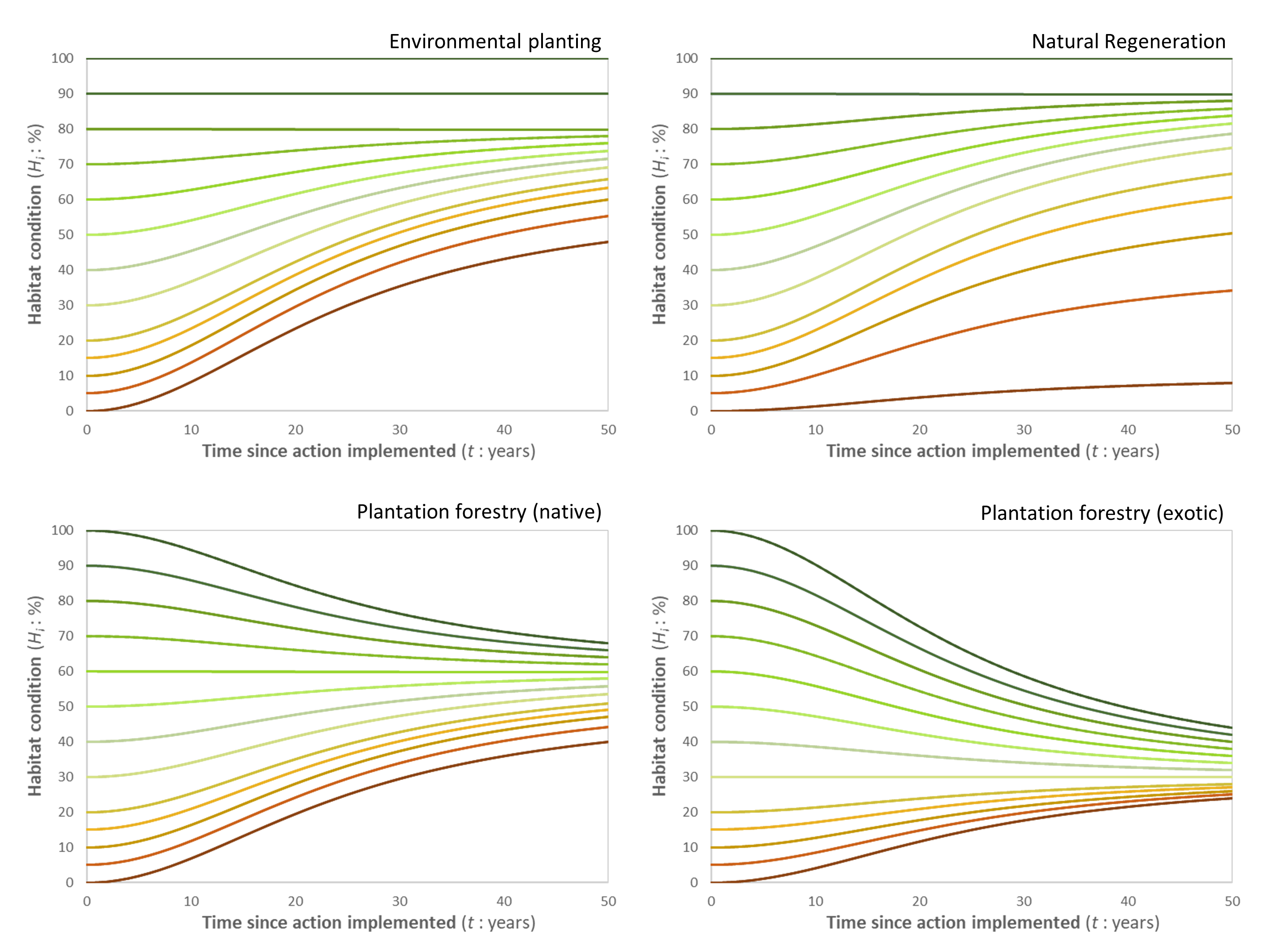
Figure 1. Graphical depiction of the forecasted changes in habitat condition for four different carbon farming actions, given differences in initial habitat condition (at \(t\)=0), based on the model applied (Eqs. 2,3) and the parameters selected (Table 1).

The parameters for maximum potential final habitat condition (\(v\)) and minimum potential final habitat condition (\(g\)) were selected based on a review of observed biodiversity outcomes from different tree planting actions in agricultural landscapes. This review considered published studies that measured biodiversity composition under all of three contrasting land uses within a landscape: (i) a natural (reference) system (e.g. forest or woodland); (ii) a non-woody agricultural system (crop or pasture), and; (iii) a former agricultural system that has had woody plants established on it (environmental planting or plantation forestry). From each study, data on the difference in species composition between each land use was obtained, primarily by digitizing ordination plots, but also through directly reported compositional similarities. From these observed compositional differences, we calculated the relative similarity of the woody planting to the natural reference system (\(S_{rel}\)) as:

\[ S_{rel} = 1 - \frac{d_{rp}}{d_{ra}} \]

Eq. 4

where \(d_{rp}\) is the compositional difference between the natural reference system (\(r\)) and the woody planting (\(p\)), and \(d_{ra}\) is the compositional difference between the natural reference system (\(r\)) and the agricultural system (\(a\)).

We restricted the data to studies from Australia and for woody plantings that were ≥ 10 years old. The average relative similarity (\(S_{rel}\)) of environmental plantings to the natural reference system was 0.36 (n = 13, SD = 0.25)^{14 15 16 17 18 19 20 21 22 23}. The average relative similarity (\(S_{rel}\)) of native plantation forestry to the natural reference system was 0.27 (n = 3, SD = 0.27)^{24 25}. There were insufficient data to obtain the average relative similarity for exotic plantation forestry ≥ 10 years old, and we did not review studies considering natural regeneration.

To apply the average relative similarities obtained from the literature review in parameterising the models of changes in habitat condition over time following implementation of carbon farming actions (Eqs. 2, 3, Table 1), we set the maximum potential final habitat condition (\(v\)) and minimum potential final habitat condition (\(g\)) values such that the estimated habitat condition at \(t = 25\) years (\(H_{i}^{t=25}\)) was as predicted by the given \(S_{rel}\) value and the habitat condition at \(t = 0\) (\(H_{i}^{t=0}\)):

\[ H_{i}^{t=25} = H_{i}^{t=0} + (S_{rel}(100 - H_{i}^{t=0})) \]

Eq. 5

For the carbon farming actions where data were not available (exotic plantation forestry, natural regeneration), the habitat condition model parameters (Table 1) were estimated based on expert judgement, in the context of the parameters derived for environmental plantings and native plantation forestry.

Habitat connectivity

Habitat connectivity is the connectedness of each location (grid cell) to natural habitat in the surrounding landscape²⁶. Habitat connectivity values range between 0 and 1.0, where a value of 1.0 indicates the grid cell is in an intact reference state and is fully connected to a landscape where all other locations are also in an intact reference state. A habitat connectivity value of 0 indicates that the grid cell has no connectivity to any locations in the surrounding landscape with any value as habitat.

To assess the connectivity of habitat, the sole input are the habitat condition data. We use an approach that considers the easiest way for species to move across the landscape given the spatial configuration of habitat condition values^{26 27}. Connectivity is higher when habitat is connected by continuous areas of habitat in good condition.

Connectivity is measured through an enhanced implementation of the cost-benefit approach15. The landscape around each grid cell is defined by a continuous measure of habitat condition, where the condition score can be interpreted as a measure of effective area (such that two grid cells of condition=0.5 are equivalent to one grid cell of condition=1). Habitat condition defines the benefit of being connected to a given grid cell, but also defines the permeability of the landscape, which can be combined with a path length to generate a cost of being connected to a given grid cell.

The metric of connectivity is calculated for each grid cell using a radial grid centred on the focal cell²⁶, extending to a radius of 100 km. Each segment of this grid is composed of multiple grid cells. The benefit of being connected to any of these segments is taken as the sum of all condition values within the segment. This is equivalent to summing the area of intact habitat in a binary intact/degraded view of condition. The effect of the permeability of each segment is calculated from the mean condition of the segment.

Biodiversity persistence

Biodiversity persistence is the number (or proportion) of species within the specified area that are expected to persist over the long term.

Biodiversity persistence in the area of interest in a specified year is estimated based on habitat condition and biodiversity patterns using the approach described by Simon Ferrier et al.²⁸, and subsequently applied in a range of studies^{29 30 31 32}. The objective of this analysis is to estimate the proportion of those species originally occurring in the area of interest that are expected to persist indefinitely into the future given the habitat condition across their entire range.

This is a community-level approach to biodiversity assessment, which has the following inputs in addition to a polygon specifying the area of interest:

• A spatial habitat condition layer for each time point of interest: derived as discussed above.

• Spatial layers from a generalised dissimilarity model (GDM)³³ estimating the level of species-assemblage similarity between pairs of locations expected if these locations were still in reference condition (i.e. the highest possible level of ecological integrity. Here we apply a GDM for vascular plants across Australia, that was derived using data from 118,509 plant community survey plots and projected at ~100 m resolution (Deviance explained = 32.4% using 8 environmental predictors and geographic distance).

• A spatial layer of expected species richness under reference habitat conditions. We use a species richness model for vascular plants across Australia that was derived using data from 118,509 plant community survey plots and projected at ~100 m resolution (Deviance explained = 33.4% using 9 environmental predictors).

The predicted pre-European spatial patterns in both species richness and pairwise compositional dissimilarity are used to estimate the total proportion of species likely to persist over a specified area at a time point (\(P\)). Specifically, for each and every ≈100 m grid cell \(i\) across Australia, we estimate the proportion (\(p_i\)) of species historically occurring in this cell (pre-European) that are likely to persist within remaining habitat anywhere in their range:

\[ pi = \left[ \frac{\sum_{j=1}^n s_{ij}h_j}{\sum_{j=1}^n s_{ij}} \right]^z \]

where \(s_{ij}\) is the predicted compositional similarity between the focal cell \(i\) and each \(j\) grid cell in the region of n grid cells, \(h_j\) is the condition of habitat in each grid cell \(j\) (ranging continuously from pristine (= 1) to completely degraded habitat (= 0)), and \(z\) is the exponent of the species–area relationship. For grid cell \(i\), \(\sum s_{ij}\) quantifies the amount of similar habitat across the region if all grid cells were in pristine condition, while \(\sum s_{ij}h_j\) quantifies the amount of similar habitat across the region, accounting for habitat loss and degradation in some grid cells (through \(h_j\)). In terms of habitat condition, the term ‘pristine’ equates to a reference state. A \(z\)-value of 0.25 was applied, which approximates values commonly observed for terrestrial taxa³⁴.

The overall proportion of species (\(P\)) expected to persist across a region can then be estimated as a weighted average of the \(p_i\) values for all n individual grid cells, to incorporate the effects of compositional overlap between grid cells and the species richness of each cell (\(r_i\)):

\[ P \frac {\sum_{i=1}^n p_iw_i} {\sum_{i=1}^n w_i} \]

where the weight (\(w_i\)) of a grid cell is calculated as:

\[ w_i = \frac{r_i}{\sum_n^{j=1} s_ij} \]

This approach is applied to estimate the proportion of the original species present that are expected to persist, given spatial patterns in habitat condition.

To translate the proportion of original species persisting into an expected number of original species persisting, we multiply the proportion by an estimate of the number of species expected to have originally occurred in the selected area. The number of species expected to have originally occurred within any specified area (1-100,000 ha) centered around each location in Australia was modelled as a function of environmental variables. Specifically, we modelled the species-area scalar (\(z\)) from the species-area power model:

\[ S = cA^z \]

where \(S\) in the number of species expected in a specified area (\(A\)), while \(c\) is the expected number of species in a unit area (here = 1 ha). For our application, we used the predicted species richness described above to define the value of \(c\) in each location. Around each location of known community composition, we derived estimates of the number of species observed (using all available occurrence data from the Atlas of Living Australia) within circular areas of increasing radii (1-100,000 ha), estimating total richness from recorded occurrences using the Chao1 species richness estimator, then using these estimates to derive the species-area scalar (\(z\)) that best fit the data. The species area scalar was then modelled using generalized additive modelling as a function of ten spatial environmental predictors (deviance explained = 19.7 %) and projected across Australia.

Threatened species habitat provision

The contribution of habitat in a specified area to supporting nationally listed threatened species is determined by calculating the number of ‘species hectares’ of habitat being provided. For each location (grid cell), the provision of habitat for threatened species is determined by multiplying the number of threatened species that may occur in that location by the estimated habitat condition in that location, where the habitat condition is 50 % or greater. Locations with lower habitat condition values (< 50 %) are assumed to provide no value for supporting threatened species. Summing the habitat provision across all locations in the specified area provides an estimate of the ‘species hectares’ of habitat being provided to nationally listed threatened species, accounting for the condition of the habitat.

To identify locations that could potentially be suitable habitat for each of Australia’s nationally listed terrestrial threatened species (excluding migratory species), we refined the ‘may occur’ spatial distribution information³⁵ provided by the Australian Department of Climate Change, Energy, the Environment and Water (DCCEEW). For each species (n = 1,466), we restricted areas within the ‘may occur’ distribution³⁵ using filtered occurrence observations from the Atlas of Living Australia³⁶, retaining only those grid cells that were within the observed elevational limits of the occurrence data, and retaining only those grid cells where the combined IBRA bioregion³⁷ and NVIS pre-European major vegetation type¹³ were represented in the occurrence observations. These refinements reduced the number of grid cells identified as potentially suitable habitat for each nationally listed threatened species, compared to the DAWE ‘may occur’ distributions³⁵, to those most likely to support those species.

We calculated the habitat provision for threatened species (in ‘species hectares’) for every 100 m grid cell across Australia, for every year. To estimate the habitat provision for threatened species into the future under forecast habitat restoration and improvement in habitat condition, the same methodology is applied, using the new estimates of habitat condition and the same spatial distributions of potential habitat for threatened species.

References

---

1. Williams KJ, Donohue RJ, Harwood TD, Lehmann EA, Lyon P, Dickson F, Ware C, Richards AE, Gallant J, Storey RJL, Pinner L, Ozolins M, Austin J, White M, McVicar TR, Ferrier S (2020) Habitat Condition Assessment System: developing HCAS version 2.0 (beta). A revised method for mapping habitat condition across Australia. Publication number EP21001. CSIRO, Canberra, Australia. https://doi.org/10.25919%2F85f4-1k65 ↩

2. DISER (2021) National forest and sparse woody vegetation data (Version 5.0 - 2020 Release). Department of Industry, Science, Energy and Resources, Commonwealth of Australia, Canberra. https://data.gov.au/data/dataset/national-forest-and-sparse-woody-vegetation-data-version-5-2020-release ↩

3. Giglio, L., Justice, C., Boschetti, L., Roy, D. (2015). MCD64A1 MODIS/Terra+Aqua Burned Area Monthly L3 Global 500m SIN Grid V006 [Data set]. NASA EOSDIS Land Processes DAAC. Accessed from https://doi.org/10.5067/MODIS/MCD64A1.006 ↩

4. ABARES (2016) Australia’s plantations 2016 dataset. Australian Bureau of Agricultural and Resource Economics and Sciences – (ABARES). https://www.agriculture.gov.au/abares/forestsaustralia/forest-data-maps-and-tools/spatial-data/australias-plantations ↩

5. Geoscience Australia (2006) GEODATA TOPO 250K Series 3 Topographic Data. Geoscience Australia. http://www.ga.gov.au:88/newintranet/meta/ANZCW0703005458.html ↩

6. Donohue, R.J., Mokany, K., McVicar, T.R., and O'Grady, A.P. (2022) Identifying management-driven dynamics in vegetation cover: applying the Compere framework to Cooper Creek, Australia. Ecosphere 13: e4006. https://doi.org/10.1002/ecs2.4006 ↩↩

7. Geoscience Australia (2021) Geoscience Australia Landsat Fractional Cover Percentiles Collection 3. Geoscience Australia. https://data.dea.ga.gov.au/?prefix=derivative/ga_ls_fc_pc_cyear_3/ ↩

8. Gallant, J. and Austin, J. M. (2012) Topographic Wetness Index derived from 1" SRTM DEM-H. v2. CSIRO Data Collection. https://doi.org/10.4225/08/57590B59A4A08 ↩

9. Gallant, J. and Austin, J. M. (2015) Derivation of terrain covariates for digital soil mapping in Australia. Soil Research 53: 895-906. ↩

10. Viscarra Rossel, R.A., Chen, C., Grundy, M.A. Searle, R., Clifford, D. and Campbell P.H. (2015) The Australian three-dimensional soil grid: Australia’s contribution to the GlobalSoilMap project. Soil Research 53: 845-864. https://doi.org/10.1071/SR14366 ↩

11. Wilford, J.R. and Kroll, A. (2019) Complete Radiometric Grid of Australia (Radmap) v4 2019 with modelled infill. Geoscience Australia. https://dev.ecat.ga.gov.au/geonetwork/srv/api/records/144413 ↩

12. Xu, T., & Hutchinson, M. (2010). ANUClim Version 6.1 User Guide. Fenner School of Environment and Society, The Australian National University Canberra. ↩

13. NVIS (2020) National Vegetation Information System (NVIS) Australia - Pre-1750 Major Vegetation Subgroups - NVIS Version 6.0 (Albers 100m analysis product). Australian Government Department of Climate Change, Energy, the Environment and Water. http://environment.gov.au/fed/catalog/search/resource/details.page?uuid=%7B418748C8-95B9-4C52-9F23-CB09E1B3D950%7D ↩↩

14. Catterall, C.P., Kanowski, J., Wardell-Johnson, G.W., Proctor, H., Reis, T., Harrison, D., Tucker N.I.J. (2004) Quantifying the biodiversity values of reforestation: perspectives, design issues and outcomes in Australian rainforest landscapes. In: (Ed. Lunney, D.) Conservation of Australia’s Forest Fauna. Royal Zoological Society of New South Wales, Mosman. pp 359-393. ↩

15. Gibb, H., Cunningham, S.A. (2010) Revegetation of farmland restores function and composition of epigaeic beetle assemblages. Biological Conservation, 143: 677-687. https://doi.org/10.1016/j.biocon.2009.12.005. ↩

16. Kinross, C. (2004). Avian use of farm habitats, including windbreaks, on the New South Wales Tablelands. Pacific Conservation Biology, 10: 180-192. https://doi.org/10.1071/PC040180. ↩

17. Law, B. S., Chidel, M. (2006) Eucalypt plantings on farms: Use by insectivorous bats in south-eastern Australia. Biological Conservation, 133: 236-249. https://doi.org/10.1016/j.biocon.2006.06.016 ↩

18. Lawes, M.J., Moore, A.M., Andersen, A.N., Preece, N.D., Franklin, D.C. (2017) Ants as ecological indicators of rainforest restoration: Community convergence and the development of an Ant Forest Indicator Index in the Australian wet tropics. Ecology and Evolution, 7: 8442-8455. https://doi.org/10.1002/ece3.2992 ↩

19. Martin, W.K., Eyears-Chaddock, M., Wilson, B.R., Lemon, J. (2004) The value of habitat reconstruction to birds at Gunnedah, New South Wales, Emu - Austral Ornithology, 104: 177-189. https://doi.org/10.1071/MU02053 ↩

20. Martin, W.K., Eldridge, D., Murray, P. (2011). Bird assemblages in remnant and revegetated habitats in an extensively cleared landscape, Wagga Wagga, New South Wales. Pacific Conservation Biology, 17: 110-120. https://doi.org/110-120. 10.1071/PC110110. ↩

21. Parkhurst, T., Prober, S.M., Standish, R.J. (2021a). Recovery of woody but not herbaceous native flora 10 years post old-field restoration. Ecological Solutions and Evidence, 2: e12097. https://doi.org/10.1002/2688-8319.12097 ↩

22. Parkhurst, T., Standish, R., Andersen, A., Prober, S. (2021b). Old‐field restoration improves habitat for ants in a semi‐arid landscape. Restoration Ecology, e13605. https://doi.org/10.1111/rec.13605. ↩

23. Smith, G.C., Lewis, T., Hogan, L.D. (2015) Fauna community trends during early restoration of alluvial open forest/woodland ecosystems on former agricultural land. Restoration Ecology, 23: 787-799. https://doi.org/10.1111/rec.12269 ↩

24. Borsboom, A.C., Wang, J., Lees, N., Mathieson, M., Hogan, L. (2002) Measurement and integration of fauna biodiversity values in Queensland agroforestry systems. Rural Industries Research and Development Corporation, Barton. ↩

25. Munro, N.T., Fischer, J., Wood, J., Lindenmayer, D.B. (2009). Revegetation in Agricultural Areas: The Development of Structural Complexity and Floristic Diversity. Ecological Applications, 19: 1197–1210. http://www.jstor.org/stable/40347262 ↩

26. Ferrier, S., Harwood, T.D., Ware, C., Hoskins, A.J. (2020) A globally applicable indicator of the capacity of terrestrial ecosystems to retain biological diversity under climate change: The bioclimatic ecosystem resilience index. Ecological Indicators, 117, 106554. https://doi.org/10.1016/j.ecolind.2020.106554 ↩↩↩

27. Drielsma, M., Ferrier, S., & Manion, G. (2007). A raster-based technique for analysing habitat configuration: The cost-benefit approach. Ecological Modelling, 202(3-4), 324-332. https://doi.org/10.1016/j.ecolmodel.2006.10.016 ↩

28. Ferrier, S., Powell, G. V. N., Richardson, K. S., Manion, G., Overton, J. M., Allnutt, T. F., . . . Van Rompaey, R. (2004). Mapping more of terrestrial biodiversity for global conservation assessment. Bioscience, 54(12), 1101-1109. ↩

29. Allnutt, T. F., Ferrier, S., Manion, G., Powell, G. V. N., Ricketts, T. H., Fisher, B. L., . . . Rakotondrainibe, F. (2008). A method for quantifying biodiversity loss and its application to a 50-year record of deforestation across Madagascar. Conservation Letters, 1(4), 173-181. https://doi.org/10.1111/j.1755-263X.2008.00027.x ↩

30. UNEP-WCMC. (2016). Exploring approaches for constructing Species Accounts in the context of the SEEA-EEA. United Nations Environment Program - World Conservation Monitoring Centre, Cambridge. ↩

31. Di Marco, M., Harwood, T. D., Hoskins, A. J., Ware, C., Hill, S. L. L., & Ferrier, S. (2019). Projecting impacts of global climate and land-use scenarios on plant biodiversity using compositional-turnover modelling. Global Change Biology, 25(8), 2763-2778. https://doi.org/10.1111/gcb.14663 ↩

32. Mokany, K., Harwood, T. D., & Ferrier, S. (2019). Improving links between environmental accounting and scenario-based cumulative impact assessment for better-informed biodiversity decisions. Journal of Applied Ecology, 56(12), 2732-2741. https://doi.org/10.1111/1365-2664.13506 ↩

33. Ferrier, S., Manion, G., Elith, J., & Richardson, K. (2007). Using generalized dissimilarity modelling to analyse and predict patterns of beta diversity in regional biodiversity assessment. Diversity and Distributions, 13, 252-264. https://doi.org/10.1111/j.1472-4642.2007.00341.x ↩

34. Rosenzweig, M. L. (1995). Species Diversity in Space and Time. Cambridge: Cambridge University Press. ↩

35. DAWE. 2022. Australia - Species of National Environmental Significance Distributions (public grids). Commonwealth of Australia (Department of Agriculture, Water and the Environment). http://www.environment.gov.au/fed/catalog/search/resource/details.page?uuid=%7B337B05B6-254E-47AD-A701-C55D9A0435EA%7D ↩↩↩

36. Atlas of Living Australia (2022) Atlas of Living Australia. https://www.ala.org.au/ ↩

37. Thackway R. & Cresswell, I.D. (1995) An Interim Biogeographic Regionalisation for Australia: A framework for establishing the national system of reserves. Australian Nature Conservation Agency, Canberra. ↩